Overview
SNP-Slice is a Bayesian nonparametric method for resolving multi-strain infections using slice sampling with stick-breaking construction. The algorithm simultaneously unveils strain haplotypes and links them to hosts from sequencing data.
This vignette demonstrates how to use SNP-Slice with the negative binomial model using real example data.
Installation
# Install from CRAN (when available)
install.packages("snp.slicer")

# Or install from GitHub
devtools::install_github("plasmogenepi/snp.slice")
Quick start
Load the package, example data, and pre-computed results:
library(snp.slicer)

# Example data: read count matrices (hosts × SNPs)
data(example_snp_data, package = "snp.slicer")
read0 <- example_snp_data$read0
read1 <- example_snp_data$read1
cat("Data dimensions:", nrow(read0), "hosts ×", ncol(read0), "SNPs\n")
#> Data dimensions: 200 hosts × 96 SNPs

# Pre-computed results (negative binomial model, 2000 MCMC iterations)
result <- load_example_results()
cat("Pre-computed results loaded successfully!\n")
#> Pre-computed results loaded successfully!

# Basic inspection
print(result)
#> SNP-Slice Results
#> ================
#> Model: negative_binomial
#> Dimensions: 200 hosts x 96 strains x 96 SNPs
#> Strains identified: 49
#> Gap Converged: No
summary(result)
#> SNP-Slice Results Summary
#> ========================
#>
#> Model: negative_binomial
#> Data dimensions: 200 hosts x 96 SNPs
#> Data type: read_counts
#>
#> Results:
#> - Number of strains identified: 49
#> - Number of hosts: 200
#> - Multiplicity of infection (MOI):
#>   - Mean MOI: 2.58
#>   - Median MOI: 1
#>   - Range: 1 - 9
#>   - Single infections: 105 ( 52.5 %)
#>   - Mixed infections: 95 ( 47.5 %)
#>
#> Convergence:
#> - Iterations run: 2000
#> - Gap Converged: No
#> - Final log posterior: -76326.7
#> - MAP log posterior: -76280.6
#> - Final k*: 113
#> - MAP k*: 113
Understanding results
The main outputs are the allocation matrix (hosts × strains) and the dictionary matrix (strains × SNPs). Use the extractors for convenience:
# Strain and allocation summaries
strains <- extract_strains(result)
allocations <- extract_allocations(result)

cat("Strains identified:", strains$n_strains, "| SNPs:", strains$n_snps, "\n")
#> Strains identified: 49 | SNPs: 96
cat("Hosts:", allocations$n_hosts, "\n")
#> Hosts: 200
cat("Multiplicity of infection (MOI) summary:\n")
#> Multiplicity of infection (MOI) summary:
print(summary(allocations$multiplicity_of_infection))
#>    Min. 1st Qu.  Median    Mean 3rd Qu.    Max.
#>   1.000   1.000   1.000   2.585   4.000   9.000

# Key matrices (also available as result$allocation_matrix, result$dictionary_matrix)
A <- result$allocation_matrix   # Hosts × Strains
D <- result$dictionary_matrix   # Strains × SNPs

cat("Allocation matrix:", dim(A), "| Dictionary matrix:", dim(D), "\n")
#> Allocation matrix: 200 49 | Dictionary matrix: 49 96
print("Sample allocation (first 3 hosts, first 5 strains):")
#> [1] "Sample allocation (first 3 hosts, first 5 strains):"
print(A[1:3, 1:5])
#>      [,1] [,2] [,3] [,4] [,5]
#> [1,]    1    0    0    0    0
#> [2,]    0    1    0    0    0
#> [3,]    1    0    0    0    0
print("Sample dictionary (first 3 strains, first 8 SNPs):")
#> [1] "Sample dictionary (first 3 strains, first 8 SNPs):"
print(D[1:3, 1:8])
#>      site1 site2 site3 site4 site5 site6 site7 site8
#> [1,]     1     1     1     1     1     1     1     1
#> [2,]     1     1     1     1     1     1     0     1
#> [3,]     1     1     0     1     1     1     0     1
Downstream analyses
Posterior allele frequencies
Compute allele (or haplotype) frequencies for specific SNP sets from
the MAP or MCMC results. Use calculate_allele_frequencies
for a single set; use calculate_allele_frequencies_by_sets
for multiple sets at once. With MAP you get point estimates and literal
counts (allele, frequency, count,
total_parasites). With MCMC you get a posterior mean
frequency, SD, credible interval, and per-sample mean count
(mean_count, n_samples), so the table does not
depend on how many MCMC samples were used.
# Single target set: allele frequencies for SNPs 1, 5, and 10 (MAP)
allele_freqs <- calculate_allele_frequencies(result, c(1, 5, 10))
head(allele_freqs)
#>        allele  frequency count total_parasites
#> 8 ref|ref|ref 0.64216634   332             517
#> 2 ref|alt|alt 0.14893617    77             517
#> 3 alt|ref|alt 0.07350097    38             517
#> 4 ref|ref|alt 0.06576402    34             517
#> 7 alt|ref|ref 0.03675048    19             517
#> 5 alt|alt|ref 0.02514507    13             517

# With MCMC: posterior mean, SD, credible interval, and sample-size-invariant mean_count
if (!is.null(result$mcmc_samples)) {
  allele_freqs_mcmc <- calculate_allele_frequencies(result, c(1, 5, 10), use_map = FALSE, n_samples = 50)
  head(allele_freqs_mcmc)
}
#>                  allele  frequency frequency_sd frequency_lower frequency_upper
#> ref|ref|ref ref|ref|ref 0.65713963  0.020364148      0.64025103      0.71437570
#> ref|alt|alt ref|alt|alt 0.13666759  0.009814729      0.10973572      0.14966914
#> alt|ref|alt alt|ref|alt 0.07438880  0.004310763      0.06658317      0.08395745
#> ref|ref|alt ref|ref|alt 0.06019152  0.008447611      0.03980544      0.06847754
#> alt|ref|ref alt|ref|ref 0.03728839  0.003938912      0.02994999      0.04316459
#> alt|alt|ref alt|alt|ref 0.01476765  0.007931272      0.00000000      0.02552901
#>             mean_count n_samples
#> ref|ref|ref     329.82        50
#> ref|alt|alt      68.74        50
#> alt|ref|alt      37.36        50
#> ref|ref|alt      30.32        50
#> alt|ref|ref      18.74        50
#> alt|alt|ref       7.48        50

# Multiple target sets: pass a named list for one table per set
target_sets <- list(
  locus_a = c(1, 5),
  locus_b = c(10, 15),
  locus_c = c(20)
)
freqs_by_set <- calculate_allele_frequencies_by_sets(result, target_sets)
# Each element is a frequency table (MAP: allele, frequency, count, total_parasites; MCMC: adds frequency_sd, frequency_lower, frequency_upper, mean_count, n_samples)
print(freqs_by_set$locus_a)
#>    allele  frequency count total_parasites
#> 4 ref|ref 0.70793037   366             517
#> 2 ref|alt 0.15667311    81             517
#> 3 alt|ref 0.11025145    57             517
#> 1 alt|alt 0.02514507    13             517
Individual COI with uncertainty
Per-host complexity of infection (COI) is the number of distinct
strains per host. Use calculate_individual_coi() for a
point estimate (MAP) or, when MCMC samples were stored, posterior mean,
SD, and a credible interval.
# Point estimate only (from MAP allocation)
coi_map <- calculate_individual_coi(result, use_map = TRUE)
head(coi_map)
#>   host_index    host_id coi_estimate coi_sd coi_lower coi_upper
#> 1          1 specimen_1            1     NA        NA        NA
#> 2          2 specimen_2            1     NA        NA        NA
#> 3          3 specimen_3            1     NA        NA        NA
#> 4          4 specimen_4            1     NA        NA        NA
#> 5          5 specimen_5            1     NA        NA        NA
#> 6          6 specimen_6            1     NA        NA        NA

# With posterior uncertainty (requires store_mcmc = TRUE)
if (!is.null(result$mcmc_samples)) {
  coi_post <- calculate_individual_coi(result, use_map = FALSE, n_samples = 50, interval = 0.95)
  head(coi_post)
  cat("\nSummary of COI posterior SD:\n")
  print(summary(coi_post$coi_sd))
}
#>
#> Summary of COI posterior SD:
#>    Min. 1st Qu.  Median    Mean 3rd Qu.    Max.
#> 0.00000 0.00000 0.00000 0.05486 0.00000 1.08965Parameter Tuning
You can adjust various parameters to optimize performance:
# Custom parameters
result_tuned <- snp_slice(data,
                         alpha = 1.5,        # IBP concentration parameter
                         rho = 0.3,          # Dictionary sparsity
                         threshold = 0.005,  # Single infection threshold
                         n_mcmc = 2000,
                         burnin = 500,       # Custom burn-in
                         gap = 10,           # Early stopping threshold
                         seed = 456,         # Reproducibility
                         verbose = FALSE)
Convergence diagnostics
When you store MCMC samples (store_mcmc = TRUE), you can
assess convergence with effective sample size (ESS) and trace plots:
if (!is.null(result$mcmc_samples)) {
  # Effective sample size for log posterior
  ess_logpost <- effective_sample_size(result, parameter = "logpost")
  ess_val <- if (is.numeric(ess_logpost)) ess_logpost else ess_logpost$ess
  cat("Effective sample size (log posterior):", round(ess_val, 1), "\n")

  # Trace plot of log posterior
  plot_convergence(result, type = "logpost")
} else {
  cat("MCMC samples not stored in results (set store_mcmc = TRUE when running snp_slice)\n")
}
#> Effective sample size (log posterior): 18.5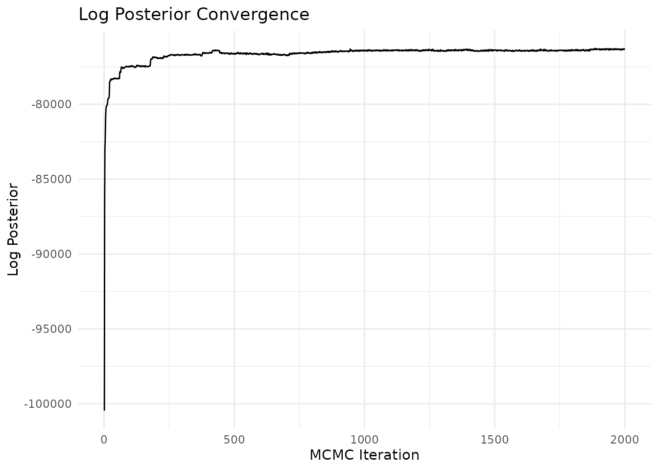
You can also use
plot_convergence(result, type = "kstar") for the number of
active strains or type = "n_strains" for strain count over
iterations. See ?effective_sample_size and
?plot_convergence for options.
Visualizing results
Let’s create some informative plots to better understand the analysis results:
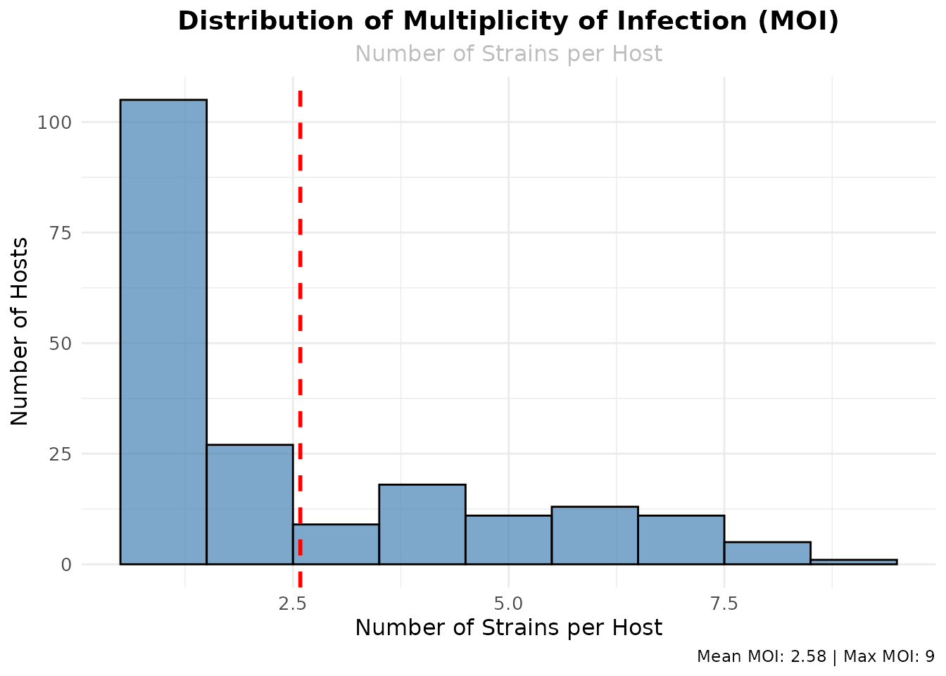
Multiplicity of Infection (MOI) Distribution
# Get MOI from allocations (same as strain diversity)
allocations <- extract_allocations(result)
moi_df <- data.frame(
  moi = allocations$multiplicity_of_infection,
  host_id = 1:length(allocations$multiplicity_of_infection)
)

ggplot(moi_df, aes(x = moi)) +
  geom_histogram(binwidth = 1, fill = "steelblue", alpha = 0.7, color = "black") +
  geom_vline(aes(xintercept = mean(moi)), color = "red", linetype = "dashed", linewidth = 1) +
  labs(
    title = "Distribution of Multiplicity of Infection (MOI)",
    subtitle = "Number of Strains per Host",
    x = "Number of Strains per Host",
    y = "Number of Hosts",
    caption = paste("Mean MOI:", round(mean(moi_df$moi), 2), "| Max MOI:", max(moi_df$moi))
  ) +
  theme_minimal() +
  theme(
    plot.title = element_text(hjust = 0.5, size = 14, face = "bold"),
    plot.subtitle = element_text(hjust = 0.5, size = 12, color = "gray"),
    axis.title = element_text(size = 12),
    axis.text = element_text(size = 10)
  )
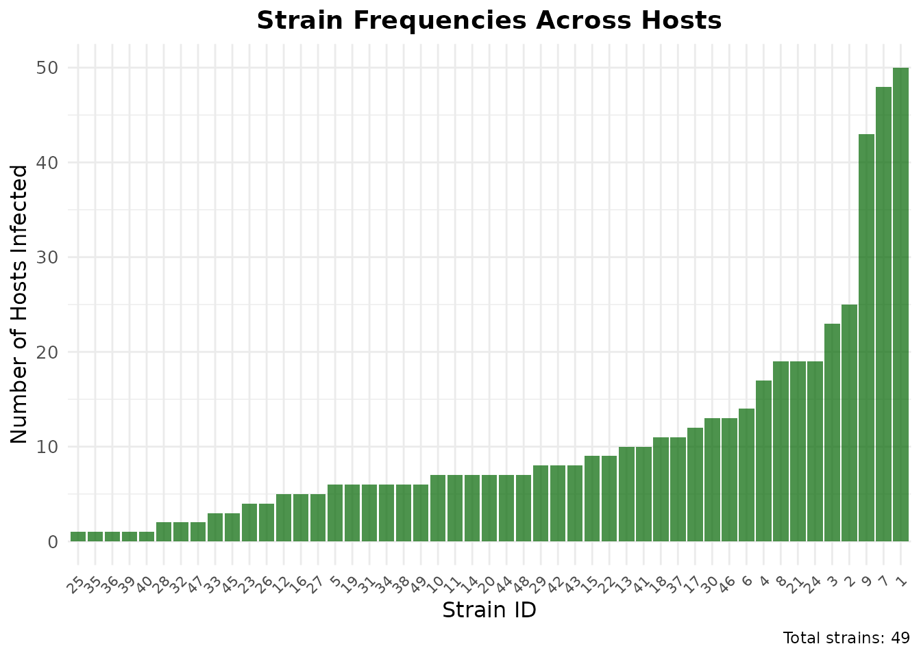
Strain Frequency Analysis
# Calculate strain frequencies
strain_frequencies <- colSums(A)
freq_df <- data.frame(
  strain_id = 1:length(strain_frequencies),
  frequency = strain_frequencies
)

# Plot strain frequencies
ggplot(freq_df, aes(x = reorder(strain_id, frequency), y = frequency)) +
  geom_bar(stat = "identity", fill = "darkgreen", alpha = 0.7) +
  labs(
    title = "Strain Frequencies Across Hosts",
    x = "Strain ID",
    y = "Number of Hosts Infected",
    caption = paste("Total strains:", length(strain_frequencies))
  ) +
  theme_minimal() +
  theme(
    plot.title = element_text(hjust = 0.5, size = 14, face = "bold"),
    axis.title = element_text(size = 12),
    axis.text.x = element_text(angle = 45, hjust = 1, size = 8),
    axis.text.y = element_text(size = 10)
  )
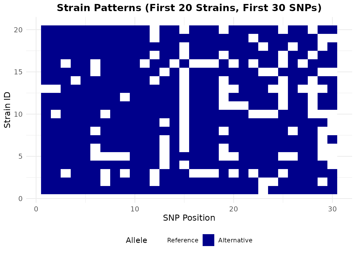
Strain Pattern Heatmap
# Create a heatmap of the first 20 strains and first 30 SNPs
D_subset <- D[1:min(20, nrow(D)), 1:min(30, ncol(D))]

# Convert to long format for ggplot
heatmap_data <- expand.grid(
  strain = 1:nrow(D_subset),
  snp = 1:ncol(D_subset)
)
heatmap_data$value <- as.vector(D_subset)

ggplot(heatmap_data, aes(x = snp, y = strain, fill = factor(value))) +
  geom_tile() +
  scale_fill_manual(
    values = c("0" = "white", "1" = "darkblue"),
    labels = c("0" = "Reference", "1" = "Alternative"),
    name = "Allele"
  ) +
  labs(
    title = "Strain Patterns (First 20 Strains, First 30 SNPs)",
    x = "SNP Position",
    y = "Strain ID"
  ) +
  theme_minimal() +
  theme(
    plot.title = element_text(hjust = 0.5, size = 14, face = "bold"),
    axis.title = element_text(size = 12),
    axis.text = element_text(size = 10),
    legend.position = "bottom"
  )
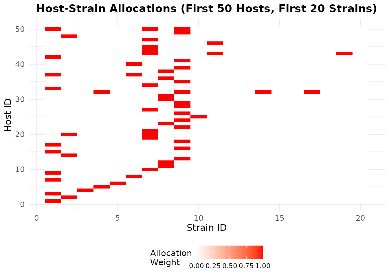
Host-Strain Allocation Heatmap
# Create a heatmap of host-strain allocations (first 50 hosts, first 20 strains)
A_subset <- A[1:min(50, nrow(A)), 1:min(20, ncol(A))]

# Convert to long format for ggplot
allocation_data <- expand.grid(
  host = 1:nrow(A_subset),
  strain = 1:ncol(A_subset)
)
allocation_data$value <- as.vector(A_subset)

ggplot(allocation_data, aes(x = strain, y = host, fill = value)) +
  geom_tile() +
  scale_fill_gradient(
    low = "white",
    high = "red",
    name = "Allocation\nWeight"
  ) +
  labs(
    title = "Host-Strain Allocations (First 50 Hosts, First 20 Strains)",
    x = "Strain ID",
    y = "Host ID"
  ) +
  theme_minimal() +
  theme(
    plot.title = element_text(hjust = 0.5, size = 14, face = "bold"),
    axis.title = element_text(size = 12),
    axis.text = element_text(size = 10),
    legend.position = "bottom"
  )
Summary Statistics
# Create summary statistics
summary_stats <- data.frame(
  Metric = c(
    "Total Hosts",
    "Total SNPs",
    "Total Strains",
    "Mean MOI",
    "Max MOI",
    "Single Infections",
    "Multiple Infections"
  ),
  Value = c(
    nrow(A),
    ncol(D),
    ncol(A),
    round(mean(allocations$multiplicity_of_infection), 2),
    max(allocations$multiplicity_of_infection),
    sum(allocations$multiplicity_of_infection == 1),
    sum(allocations$multiplicity_of_infection > 1)
  )
)

# Display summary table
knitr::kable(summary_stats,
             col.names = c("Metric", "Value"),
caption = "Summary Statistics from SNP-Slice Analysis")| Metric | Value |
|---|---|
| Total Hosts | 200.00 |
| Total SNPs | 96.00 |
| Total Strains | 49.00 |
| Mean MOI | 2.58 |
| Max MOI | 9.00 |
| Single Infections | 105.00 |
| Multiple Infections | 95.00 |
Next steps
This vignette covered the basics of using SNP-Slice with the negative binomial model. For more:
-
Other models: Try Poisson, binomial, or categorical
models via the
modelargument insnp_slice(). -
Diagnostics: Use
?effective_sample_sizeand?plot_convergencewhen MCMC samples are stored. -
Your data: Apply SNP-Slice to your own read count
or categorical data; see
?snp_sliceand?load_example_resultsfor input format and examples. -
Parameters: Fine-tune
alpha,rho,threshold,burnin, andgapfor your application.
References
- SNP-Slice Resolves Mixed Infections: Simultaneously Unveiling Strain Haplotypes and Linking Them to Hosts
- BioRxiv preprint